Nano Perceiver
Tl;dr
The Perceiver family of models from DeepMind decouple context length from memory and compute requirements. Perceiver AR extends this with support for autoregressive generation. It also has a refreshingly simple implementation, since at it’s core it is just a small variation on top of an otherwise standard decoder-only transformer.
I’ve provided a lightweight implementation here and provide additional context in this post.
Background
Notation
Let’s set some consistent notation:
- For inputs, consider
- Index (i.e., first) dimensionality as \(M\), also known as context size
- Channel (i.e., second) dimensionality as \(C\)
- For a transformer model, consider:
- A model with \(L\) transformer “blocks”, each with
- an attention layer
- a relatively shallow MLP
- A model with \(L\) transformer “blocks”, each with
For example, these inputs could be
- \(M\) token embeddings, each with an embedding size of \(C\)
- \(M\) raw pixels from a color image, with \(C = 3\) for RGB.
Transformers and scale
Transformers are increasingly powerful and expressive with increasing training data and parameter count, as demonstrated by large transformers like GPT-4 and PaLM. However, transformers scale poorly with w.r.t. both compute and memory when context size increases.
Self-attention is quadratic
The most important operation in a transformer model is the attention operation, hence the seminal paper’s title being Attention Is All You Need.
If you’re unfamiliar with attention, then there are an inordinate amount of intuitive explanations out there, but here’s my abbreviated take that highlights the scaling: At its core, self-attention tries to determine for each input token, how it relates to each other input token. This is basically a doubly nested for-loop:
def self_attention(some_inputs):
    scores = [
        [0 for _ in range(len(some_inputs))]
        for _ in range(len(some_inputs))
    ]
    for r, query_tok in enumerate(some_inputs):
        for c, key_tok in enumerate(some_inputs):
            score_qk = relation(get_query_vector(query_tok), get_key_vector(key_tok))
            scores[r][c] = score_qk
    ...  # Normalize, combine with value vectors, etc
This is obviously quadratic.
If you’re familiar with basic matrix math, you’ll observe that you can rewrite this more compactly with some matrix operations. I.e. given \(Q, K, V \in \mathbb{R}^{M \times C}\), the attention operation is:
\[\text{softmax} \left( \frac { QK^T }{\sqrt C} \right) V\]Here you can see that attention scales quadratically via observing that \(QK^T \in \mathbb{R}^{M \times M}\).
But let’s not forget about “linear” scaling either
A standard transformer has \(L\) blocks, which means both self-attention and subsequent MLP are run \(L\) times, which brings overall complexity to \(O(M^2L)\) and \(O(ML)\) for the attention and MLP operations respectively.
Suppose by some miracle we are able to reduce self-attention’s complexity down to \(O(M)\), perhaps via some clever approximations. Throwing the math under the rug of Big-O notation, this would imply that a transformer model scales with \(O(ML)\). This is of course better than \(O(M^2L)\), but for large M (e.g. long context models), this is still rather poor scaling.
This incentivizes model designers to come up with clever and bespoke ways of reducing context length (e.g. the ViT, which famously converts an image into patches first). These are effective, but it’s not always clear how to handle other domains, and it’s tremendously easy to get input sizes that are in the deep hundreds of thousands, if not larger. For example, 10 seconds of time-domain audio (\(10s \times 44.1 \text{kHz} = 441 \text{ thousand}\)) or 10 seconds of low resolution (e.g. 240p) grayscale video without any audio (\(\text{240 px high} \times \text{362 px wide} \times 24 \text{Hz} \times 10s \approx 20 \text{ million}\)).
Therefore, there’s a desire to not only handle the quadratic nature of self-attention, but also to further decouple context length from computation (past processing the inputs, of course).
Perceiver architecture
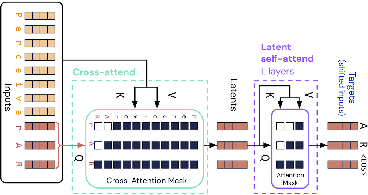
The crux of the Perceiver architecture is to use cross-attention for the first block. The only difference between cross-attention and self-attention is that cross attention uses query vectors that are attending to key and value vectors that may come from a different underlying inputs1:
\[Q \in \mathbb{R} ^ {N \times C}; \; K, V \in \mathbb{R} ^{M \times C}\]Consider \(N\) to be a hyperparameter, selected such that \(N \ll M\). Now \(QK^T \in \mathbb{R}^{N \times M}\); as in, the first attention layer is now an \(O(NM)\) operation! And, since the output latents are of length \(N\), each subsequent self atttention is \(O(N^2)\), and each MLP layer is also only \(O(N)\) now.
Getting the queries
This is all well and good, but it depends on our ability to actually get reasonable queries.
For the initial query, both the original Perceiver and Perceiver IO used a fixed latent, analogous to the initial hidden state in an RNN. Perceiver AR uses an arguably simpler approach, where the initial query just comes from the last \(N\) inputs. This way, you can still apply causal masking for autoregressive generation!
Since \(N\) is now a hyperparameter choice, if one uses \(N=M\), then this is actually equivalent to a standard decoder-only transformer, which I find particularly elegant.
Just show me the code
So conceptually this makes sense, so what do we need to actually modify? Well, as you can also see from the above diagram, there’s not too much to change. You need to
- Ensure your targets are the same size as your queries.
- Explicitly choose queries as the tail of your full context input.
- Ensure your “triangular” causal attention masking is shifted accordingly.
Targets
x = torch.stack([data[i : i + block_size] for i in ix])
y = torch.stack(
    [data[i + block_size + 1 - query_size : i + block_size + 1] for i in ix]
)
For a standard transformer, query_size is identical to block_size.
Attention module
def forward(self, inputs_q, inputs_kv):
    ...
    # Causal masking.
    mask = torch.tril(
        torch.ones(q_time, kv_time, device=attention.device),
        diagonal=kv_time - q_time,
    )
    attention = attention.masked_fill(~mask.bool(), float("-inf"))
For a standard transformer, the diagonal argument is just 0, the default value.
Perceiver block
def forward(self, x: torch.Tensor):
    inputs_q, inputs_kv = x[:, -self.query_size :, :], x
    normed_q, normed_kv = self.ln1(inputs_q), self.ln1(inputs_kv)
    x = inputs_q + self.attn(inputs_q=normed_q, inputs_kv=normed_kv)
    x = x + self.mlp(self.ln2(x))
    return x
For a standard transformer, the main Block’s forward function only passes the input to attention, since it’s doing self-attention, but since we’re now doing cross-attention on inputs, we need to handle inputs_q and inputs_kv separately.
The attention operations in the middle of the transformer are self-attentions over the \(\mathbb{R} ^ {N \times C}\) latent space, so for these layers the inputs_q == inputs_kv since getting the last the full size of the latent is just self.query_size anyways.
Is that all?
And… that’s about it. Feel free to see the full repo here.2 The repo takes inspiration (and code) from Karpathy’s NanoGPT repo, and reuses the core logic around a simple training script over a single plain text file Shakespeare “corpus”. I encourage you to mess around with some of the parameters in the train.py script. I was able to train surprisingly long context models, caveated that I was running locally on a 2019 Macbook, but of course you’re free to use a proper accelerator of your choice.
If you want to see a more fully fleshed out implementation, then you’ll be pleased to know that DeepMind has actually open sourced a repo here. It’s a research codebase so it definitely was not designed for pedagogical friendliness, but it is supremely flexible3.
Notes
-
The original Perceiver paper goes further and uses \(Q \in \mathbb{R} ^ {N \times D}\), which requires further projections. Fun fact, the original implementation refers to this projection as
conv_1deven though it’s just aLinear. I’m not exactly sure why they’d call it this; perhaps due to other patterns in computer vision where a 1x1 convolution has been used to reduce channel size? ↩ -
This repo doesn’t experiment with any more sophisticated optimizers, nonlinearities, or further-optimized attention chunking/computation. This repo also assumes you are not meddling with channel dimensions, e.g. not projecting into larger or smaller channel sizes. ↩
-
It’s also implemented in JAX, which is a pro or con depending on whether or not you’re a Googler (jk, kind of 🙂). ↩